In this post, we are going to see Sensitivity Analysis in Excel.
Discounted Cash flow is probably the commonest way of valuation of a company.
This method involves amongst other things analyzing the impact of factors like cost of equity or change in risk-free rate on the price of a company’s share.
It is but obvious that any company operates in a dynamic environment and hence for investors it is imperative that the model so built gives the investor a range of price movement so that they are prepared with respect to the possible price fluctuations that they might have to encounter if they decide to stay invested in the company.
Investors can gauge the sensitivity of price to various inputs using a technique called “sensitivity analysis”.
Sensitivity analysis is especially useful in cases where investors are evaluating proposals for the same industry or in cases where proposals are from multiple industries but driven by similar factors
What Is Sensitivity Analysis in Excel?
As the words suggest, in sensitivity analysis, we try and ascertain the impact of a change in outcome for changes in inputs.
In other words, it is also a function of the effect of various analysis data inputs to the outcome and also the impact that each input has.
The most common tool available for us to do sensitivity analysis is Microsoft Excel.
So How Do We Do It?
In Excel, sensitivity analysis comes under “What-if” analysis functions. The following are used most often
(1) Data Table
1. One-Variable Data Table
2. Two-Variable Data Table
(2) Goal Seek
Data Tables
1. One-Variable Data Table
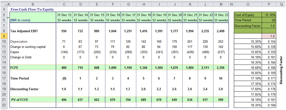
Let us assume that we would like to know the impact that any change in the cost of equity on the discounting factor which would be used to calculate the discounting factor.
Our model currently shows that the discounting factor at 15.1% cost of equity is approximately 0.97.
Now if we need to analyze the impact of change in the cost of equity on discounting factor, then we could do the following:

Steps:
a) Type the list of values that you want to evaluate in the input cell either down one column or across one row.
b) Leave a few empty rows and columns on either side of the values.
c) If the data table is column-oriented (your variable values are in a column), type the formula in the cell in a manner similar to how we have done in cell P9.
d) Select the range of cells that contains the formulas and values that you want to substitute. For us, this range is O9:P22.
e) The results i.e. incremental changes in discounting factor would automatically appear in cells P9:P22.
2. Two-Variable Data Table
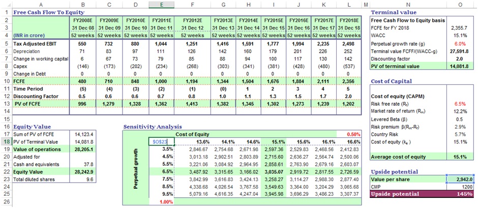
Let us take another example wherein we need to analyze the impact of change in not only cost of equity but also risk-free rate on the Value per Share.
If we need to factor in both these variables, then we would be using a two-variable data table for sensitivity analysis in Excel.

The following are the additional steps that we need to do to include the two variables:
a) Since the Excel data table has both columns and rows, hence the formula cell shifts exactly above the column variable and right beside the row variable, which for us is cell E18.
b) Select the range of cells that contains the formulas and values that you want to substitute. For us, this range is E18:L24.
c) On the Data tab, click What-If Analysis, followed by“Data Table”. Type the cell reference
- For the “Column input” cell box, for us, it’s O13.
- For the Row input cell box, for us, it’s O20.
d) The results i.e. the possible variations in would automatically appear in cells E19:L25.
Goal Seek
This function is used to find the missing input for the desired result.
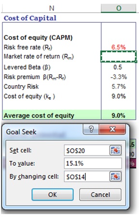
Let’s take the example of the model that we have used for Data Tables. Here let’s say we know the cost of equity.
However, we are not sure what would be the market risk premium. In this scenario “Goal Seek” is an excellent function for sensitivity analysis in Excel.

The methodology of using “Goal Seek” is as follows.
a) On the Data tab, click What-If Analysis and then click “Goal Seek”.
b) In the Set cell box, enter O20, the cell with the formula you want
in our case it’s the average cost of equity.
c) In the To value box, type the target value i.e. 15.1%.
d) In the By changing cell box, enter O14, the reference to the cell that contains the value that you want to adjust.
e) Click OK and the result would come up as 12.3% after rounding off.
I have also created a video to help you understand how to use sensitivity analysis for DCF valuation.
Thus to conclude, we can state that Excel allows us to use various tools to make our lives easier.
In financial modeling, one of the key components to efficiently perform requirements related to interpreting sensitivity is by using “What-If Analysis” with various steps as mentioned above.
Learn more about financial modeling careers.
Using Data tables and goal seek function we can save ourselves from a lot of time and error wastage that may occur in case you decide to do the calculations by hand.
In all probability, learning effective use of sensitivity analysis in Excel would make us better prepared to understand the impact of inputs on the value of investments and hence keep us better prepared for fluctuations once we commit our investments.
The use of Sensitivity Analysis using Excel in financial modeling is unarguable.
Takeaway
I am sure this guide added value to you in doing Sensitivity Analysis in Excel. If you have any queries, please leave a comment below.


Reason for that is you are giving hard punch value for the BASE COLUMN (Refer TWO variable Analysis cell E18), ideally it should be linked.
i was trying to download and see how it works How to Do DCF Valuation Using Sensitivity Analysis in Excel
OK. So, what’s the problem?
Fantastic explanation, I am wondering why I still get all the same values for my SA though, is there some complication with how excel pulls the data?