In this article, I’m going to explain how to calculate one of the most famous ratios, among financial analysis, to measure risk in Microsoft Excel: the Sharpe Ratio Excel.

The Nobel laureate William F. Sharpe developed the Sharpe Ratio.
According to Investopedia:
“The Sharpe ratio is calculated by subtracting the risk-free rate from the return of the portfolio and dividing that result by the standard deviation of the portfolio’s excess return.”
The formula is the following:

Where Expected Return (P) is the expected return of the portfolio and “Standard Deviation (P)” is the standard deviation of the portfolio’s excess return.
How to Calculate the Sharpe Ratio Excel?
Now let’s get hands-on work and calculate the Sharpe Ratio for a two – stocks portfolio in MS Excel.
For the analysis, we will suppose that our portfolio is composed of 50% by Apple Inc. (AAPL) and 50% by Microsoft Corp. (MSFT).

Step 1:
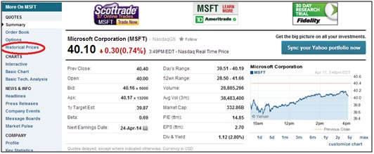
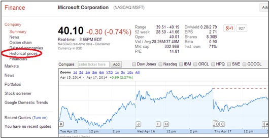
First of all, we need to get the stocks’ daily prices in order to calculate the daily returns that we are going to use to calculate the variables that compose the Sharpe Ratio.
We can get historical prices from many sources but the most famous one is Google Finance:


Step 2:
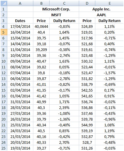
Input the daily prices into an Excel worksheet and calculate returns for the period being analyzed (I will use a 3-year time horizon).
The return can be calculated with the formula below:
Daily Return = (Price 1 – Price 0) / Price 0
Daily Return = (Price 1 / Price 0) -1
Where Price 1 is the following day close price and Price 0 is the previous day close price.

Step 3:
Once we have all the returns daily, we are able to calculate the expected return for each of the stocks. To do this, we have to calculate the average of the returns for the days period being analyzed and then annualize it.
We will use Excel’s average formula: =AVERAGE (Range of Returns1) and then we annualize it by multiplying by 252 (tradable days).
Then, we have to do the same calculations for the second stock:
=AVERAGE (Range of Returns2) and then we annualize it by multiplying by 252.
Step 4:
Following the Sharpe Ratio formula, another variable we need to calculate is the Standard Deviation of the portfolio.
Let’s remember the Variance formula for a two-stocks portfolio:
VAR (P) = Weight1^2 * STDEV1^2 + Weight2^2 * STDEV^2 +2 * Weight1 * Weight2 * STDV1 * STDV2 *CORR(1,2)
Where COV(1,2) = STDEV1 *STDEV2 * CORR1,2
So, VAR (P) = Weight1^2 * STDEV1^2 + Weight2^2 * STDEV^2 + 2 * Weight1 * Weight2 * COV1,2
Then, the standard deviation of the portfolio is the squared root of the Variance.
STDEV (P) = (Weight1^2 * STDEV1^2 + Weight2^2 * STDEV^2 + 2 * Weight1 * Weight2 * COV1,2)^(1/2)
One of the inputs we can easily calculate in Excel is the Standard Deviation of the returns of each stock:
For the first stock = STDEV1 (Range of Returns1)
For the second stock = STDEV2 (Range of Returns2).
Then, we need to calculate the Covariance of the two stocks based on the returns.
Note: According to Investopedia, the covariance is a measure of the degree to which returns on two risky assets move in tandem. A positive covariance means that asset returns move together. A negative covariance means returns move inversely.
To do this we use the covariance function provided by Excel: =COVAR (Range of Returns 1; Range of Returns2)
Once we have calculated the Standard Deviation and the Covariance of the stocks, we can put all the variables together and get the Std Deviation of the Portfolio.
The standard deviation calculated is on a daily basis and we have to get it annualized so we have to multiply the result by the squared root of 252 (average number of tradable days per year).
Step 5:
We are one step to finish the calculation! We just need to get the Risk Free Rate and put all the variables together.
The United States Treasury Bonds are known as risk-free because they always pay. For this analysis, a 5-year bond will be considered with an annual rate of 1.72%.
The numbers for the example are the following:
Annualized Expected Return MSFT= 0.07%*252 = 18.46%
Annualized Expected Return AAPL= 0.08%*252 = 19.29%
Annualized Portfolio Return= 0.5*18.46% + 0.5*19.29% = 18.87%
Std Dev MSFT= 1.49%
Std Dev AAPL= 1.77%
Covariance (MSFT, AAPL)= 0,0001
Portfolio’s Std Deviation (Daily) = (0.5^2*1.49%^2+0.5^2*1.77%^2+2*0,5*0,5*0,0001)^(1/2) = 0.02%
Portfolio’s Std Deviation (Annualized) = (0.02%*252)^(1/2)= 20.71%
Risk Free Rate= 1.72%
Putting all the variables together into the Sharpe Ratio formula we get the following:


Sharpe Ratio (P) = (18.87% – 1.72%) / 20.71% = 0.83
So, I am sure now you are clear as to how to calculate Sharpe Ratio formula in Excel.
Suggested: Read more about financial modeling careers.
Please comment below if you have any questions.


